Insights that fuel performance.
Our point of view on performance media.
Deep dives.
Making an impact means having a point of view. We engage with the biggest topics in performance marketing-looking at all sides.

Giving Growth: A podcast dedicated to issues and challenges for non-profit marketers.
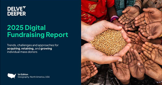
2025 Digital Fundraising Report


The Audience-First Giving Pyramid
What obsesses us.
From personalization to profitability, our insights cover the vast ground of performance media.
Point digital media funds at new-to-file and sustainers

Why digital fundraisers can’t leave marketing to marketers

Urgent Google Ads Update: How to Set Up Google Consent Mode V2 Advanced Before June 15, 2026

ChatGPT Ads Are Live. 100 Million Weekly Queries. Almost Zero Competition.

When Doing More Isn’t Enough: Recognition, Growth, and Rebuilding Connection in Today’s Workplace

When There’s No Finish Line: What Nonprofit Teams Are Actually Feeling Right Now

Rebuilding Donor Trust When Skepticism Is the Default

Lack of Personalization Is Why Monthly Donors Leave Quietly

Lack of Segmentation Keeps Your Best Donors Invisible

Inefficient Media: What Happens When Platforms Optimize Without Context
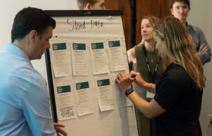
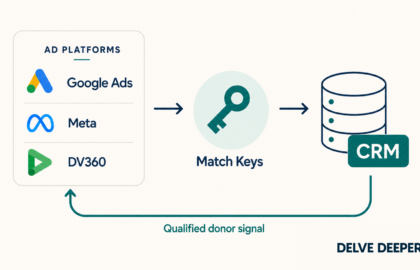
Siloed Data Is Hiding Your Best Donors
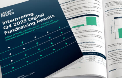
Interpreting Q4 2025 Digital Fundraising Results

Benchmark Your End-of-Year RoAS

Best creative practices for digital campaigns

Why more CMOs need to get obsessed

Rethinking the giving pyramid for a new age of philanthropy

Why the marketing funnel is dead

Decoding your superfans and distractors to unlock an unfair marketing advantage

10 tips for a winning
first-party data strategy
first-party data strategy

3 Mindset-Shifting Ways To Help Embed Personalization into Your Marketing

Why SA360 is Your AI Command Center

Why GA4 is the Only Choice for Your Measurement Foundation

Why Enterprise Advertisers Are Consolidating on DV360

Why GMP is the Ultimate Enterprise Advantage

Here’s How Marketing Leaders’ Roles Are Changing

A Recipe for Building a High-Revenue Marketing Engine

How first-party data transformation helps build competitive advantage

How CMOs Can Lead With First-Party Data